num_obs <- 30
beta0 <- 10
beta1 <- -3
sigma <- 3해당 자료는 전북대학교 이영미 교수님 2023응용통계학 자료임
예시
- y = 10 - 3x + epsilon
- epsilon ~ N(0, 3^2)
set.seed(1)
epsilon <-  rnorm(n = num_obs, mean = 0, sd = sigma)
x <- 1:num_obs
y <- beta0 + beta1*x + epsilonsim_model1 <- lm(y~x)
summary(sim_model1)
Call:
lm(formula = y ~ x)

Residuals:
    Min      1Q  Median      3Q     Max
-6.9439 -1.3193  0.3063  1.8845  4.1365

Coefficients:
            Estimate Std. Error t value Pr(>|t|)
(Intercept) 10.78911    1.05002   10.28 5.27e-11 ***
x           -3.03495    0.05915  -51.31  < 2e-16 ***
---
Signif. codes:  0 ‘***’ 0.001 ‘**’ 0.01 ‘*’ 0.05 ‘.’ 0.1 ‘ ’ 1

Residual standard error: 2.804 on 28 degrees of freedom
Multiple R-squared:  0.9895,    Adjusted R-squared:  0.9891
F-statistic: 2633 on 1 and 28 DF, p-value: < 2.2e-16plot(y ~ x, pch=16, col='darkorange')
abline(sim_model1, col='steelblue', lwd=2)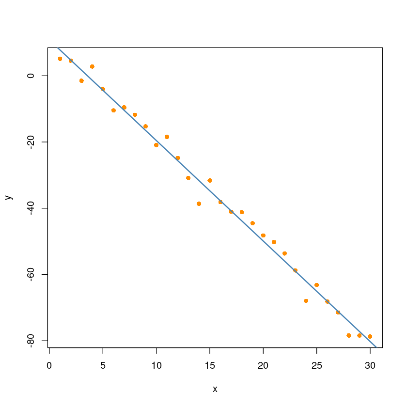
confint(sim_model1, level = 0.95)| 2.5 % | 97.5 % | |
|---|---|---|
| (Intercept) | 8.638235 | 12.939986 |
| x | -3.156107 | -2.913795 |
The function to generate simulation data
generating_slr = function(x, beta0, beta1, sigma) {
  set.seed(1)
  n = length(x)
  epsilon = rnorm(n, mean = 0, sd = sigma)
  y = beta0 + beta1 * x + epsilon
  data.frame(x,y)
}par(mfrow=c(1,2))
x <- 1:10
beta0 <- 10
beta1 <- -3
sigma <- 3sim_dat <- generating_slr(x, beta0, beta1, sigma)
sim_fit <- lm(y~x, data = sim_dat)plot(y ~ x, data = sim_dat,
pch=16, col='darkorange',
main =bquote(hat(beta)[0] ~ "="~.(beta0) ~ ", " ~
hat(beta)[1] ~ "="~.(beta1)~ ", " ~
sigma ~"="~ .(sigma)))
abline(sim_fit, col='steelblue', lwd=2)
abline(10, -3, col='red', lwd=2)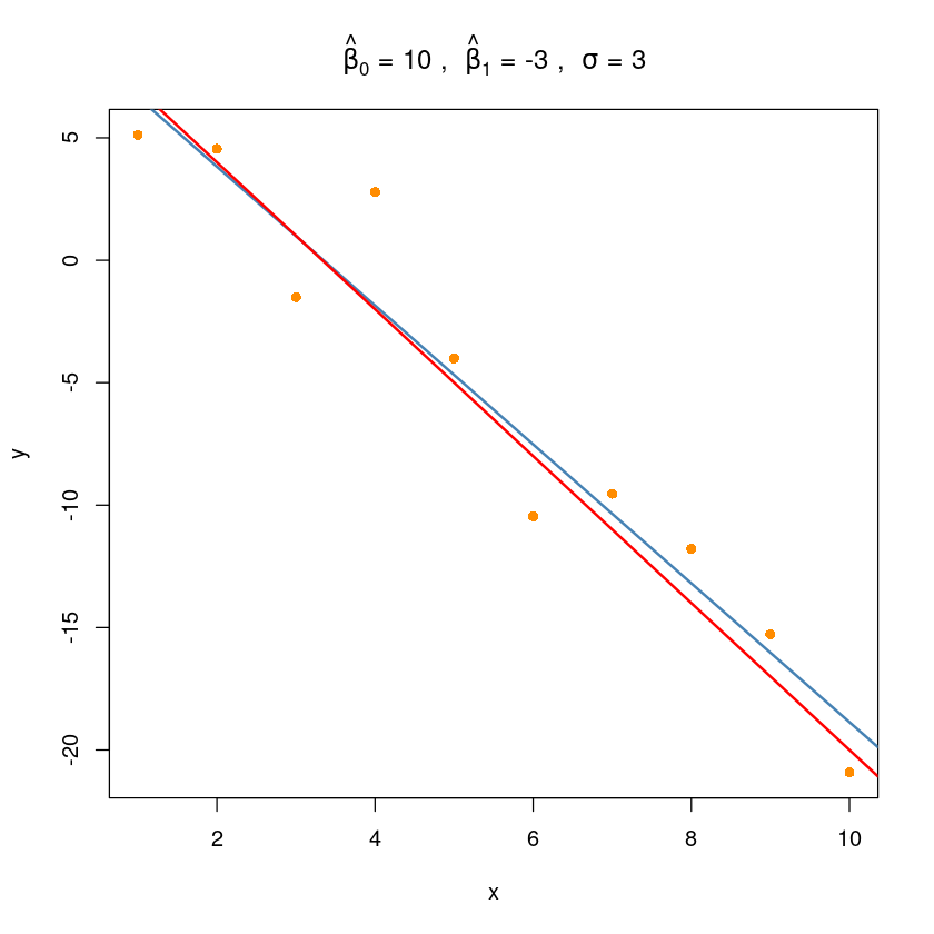
summary(sim_fit)
Call:
lm(formula = y ~ x, data = sim_dat)

Residuals:
    Min      1Q  Median      3Q     Max
-2.9401 -1.9230  0.7015  0.8036  4.6355

Coefficients:
            Estimate Std. Error t value Pr(>|t|)
(Intercept)   9.4935     1.6581   5.726 0.000441 ***
x            -2.8358     0.2672 -10.612 5.44e-06 ***
---
Signif. codes:  0 ‘***’ 0.001 ‘**’ 0.01 ‘*’ 0.05 ‘.’ 0.1 ‘ ’ 1

Residual standard error: 2.427 on 8 degrees of freedom
Multiple R-squared:  0.9337,    Adjusted R-squared:  0.9254
F-statistic: 112.6 on 1 and 8 DF,  p-value: 5.438e-06
회귀계수
hat beta0 ~ N(beta0, Var(hat beta0))
hat beta1 ~ N(beta1, Var(hat beta1))
num_samples = 10000beta0_hats = rep(0, num_samples)
beta1_hats = rep(0, num_samples)x1 <- seq(3,7, lenth.out=20)
x2 <- seq(1,10, lenth.out=20)
beta0 <- 10
beta1 <- -3
sigma <- 3Warning message:
“In seq.default(3, 7, lenth.out = 20) :
extra argument ‘lenth.out’ will be disregarded”
Warning message:
“In seq.default(1, 10, lenth.out = 20) :
extra argument ‘lenth.out’ will be disregarded”tmp_dt1 <- generating_slr(x1, beta0, beta1, sigma)
tmp_dt2 <- generating_slr(x2, beta0, beta1, sigma)par(mfrow=c(1,2))
plot(y~x, tmp_dt1)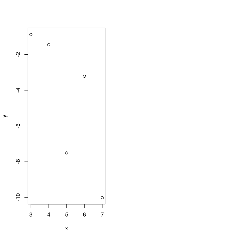
m1 <- lm(y~x, tmp_dt1)
m2 <- lm(y~x, tmp_dt2)
summary(m1)$coef
summary(m2)$coef| Estimate | Std. Error | t value | Pr(>|t|) | |
|---|---|---|---|---|
| (Intercept) | 5.402469 | 4.5800907 | 1.179555 | 0.3231998 |
| x | -2.002932 | 0.8814389 | -2.272343 | 0.1076921 |
| Estimate | Std. Error | t value | Pr(>|t|) | |
|---|---|---|---|---|
| (Intercept) | 9.493529 | 1.6580904 | 5.72558 | 4.411935e-04 |
| x | -2.835804 | 0.2672255 | -10.61203 | 5.438402e-06 |
num_samples = 10000
beta0_hats = rep(0, num_samples)
beta1_hats = rep(0, num_samples)
x <- 1:10
beta0 <- 10
beta1 <- -3
sigma <- 3

set.seed(1004)
for (i in 1:num_samples) {
  tmp_dt <- generating_slr(x, beta0, beta1, sigma)

  sim_fit = lm(y ~ x, tmp_dt)

  beta0_hats[i] = coef(sim_fit)[1]
  beta1_hats[i] = coef(sim_fit)[2]
}
## beta1
head(beta1_hats)- -2.83580381478312
- -2.83580381478312
- -2.83580381478312
- -2.83580381478312
- -2.83580381478312
- -2.83580381478312
mean(beta1_hats) ## empirical mean of beta1_hat
-2.83580381478312
beta1 ## true mean of beta1_hat
-3
var(beta1_hats) ## empirical variance of beta1_hat
0
var_beta1_hat <- sigma^2/ sum((x - mean(x))^2)  ## true variance of beta1_hat
var_beta1_hat
0.109090909090909
hist(beta1_hats, prob = TRUE, breaks = 20,
     xlab = expression(hat(beta)[1]), main = "", border = "steelblue")  ## empirical distribution of beta1_hat
curve(dnorm(x, mean = beta1, sd = sqrt(var_beta1_hat)),
      col = "darkorange", add = TRUE, lwd = 3)  ## true distribution of beta1_hat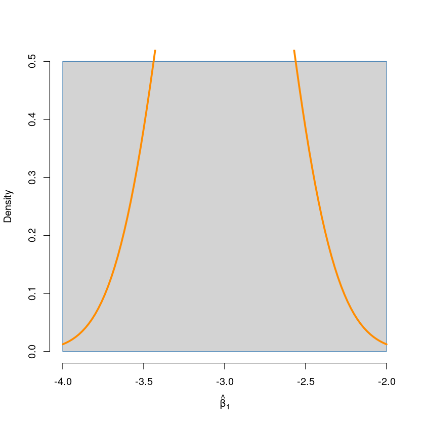
model
## Model1 : y = 3 + 5x + epsilon,  epsilon~N(0,1)
## Model2 : y = 3 + 5x + epsilon,  epsilon~N(0,x^2)
## Model3 : y = 3 + 5x^2 + epsilon, epsilon~N(0,25)- generating function
sim_1 = function(n) {
  x = runif(n = n) * 5
  y = 3 + 5 * x + rnorm(n = n, mean = 0, sd = 1)
  data.frame(x, y)
}
sim_2 = function(n) {
x = runif(n = n) * 5
y = 3 + 5 * x + rnorm(n = n, mean = 0, sd = x)
data.frame(x, y)
}sim_3 = function(n) {
x = runif(n = n) * 5
y = 3 + 5 * x ^ 2 + rnorm(n = n, mean = 0, sd = 5)
data.frame(x, y)
}
n <- 200
set.seed(1004)
dt1 <- sim_1(n)
dt2 <- sim_2(n)
dt3 <- sim_3(n)
head(dt1)| x | y | |
|---|---|---|
| <dbl> | <dbl> | |
| 1 | 1.358233 | 9.348186 |
| 2 | 1.229829 | 8.768066 |
| 3 | 3.893231 | 21.079976 |
| 4 | 4.895058 | 28.165052 |
| 5 | 2.173793 | 11.262647 |
| 6 | 4.570661 | 25.031025 |
head(dt2)| x | y | |
|---|---|---|
| <dbl> | <dbl> | |
| 1 | 3.622810 | 18.645942 |
| 2 | 1.045306 | 10.137068 |
| 3 | 3.168525 | 17.546195 |
| 4 | 3.585000 | 23.911858 |
| 5 | 3.989679 | 18.895470 |
| 6 | 1.211359 | 8.320489 |
head(dt3)| x | y | |
|---|---|---|
| <dbl> | <dbl> | |
| 1 | 4.016845 | 82.23803 |
| 2 | 3.874216 | 84.05972 |
| 3 | 2.675354 | 31.63082 |
| 4 | 4.220042 | 85.95100 |
| 5 | 3.426507 | 57.40688 |
| 6 | 2.881320 | 41.75378 |
par(mfrow=c(1,3))
plot(y~x, dt1, col='grey', pch=16, main = "Model1")
plot(y~x, dt2, col='grey', pch=16, main = "Model2")
plot(y~x, dt3, col='grey', pch=16, main = "Model3")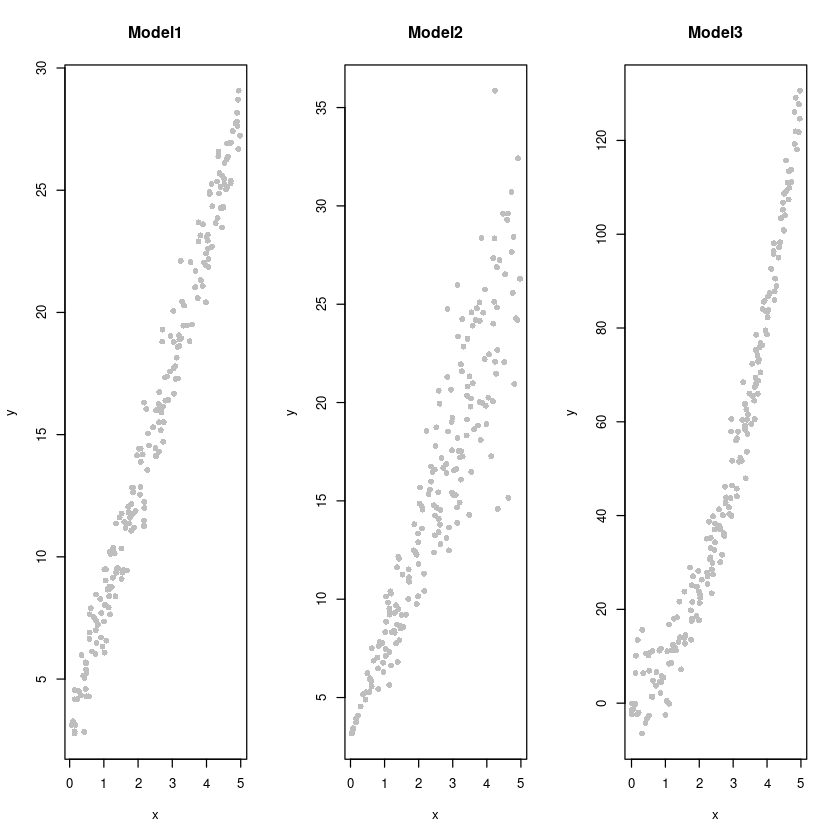
##### model fitting

fit1 <- lm(y~x, dt1)
fit2 <- lm(y~x, dt2)
fit3 <- lm(y~x, dt3)
fit4 <- lm(y~x+I(x^2), dt3)- fit4의 경우는 x^2을 추가 해서.. 사용한다.
- fit4 <- lm(y~x+I(x^2), dt3) 로 하면 된다.ㅇI 안쓰면 안된ㅁ
summary(fit3)
Call:
lm(formula = y ~ x, data = dt3)

Residuals:
    Min      1Q  Median      3Q     Max
-18.526  -8.086  -1.802   6.021  27.172

Coefficients:
            Estimate Std. Error t value Pr(>|t|)
(Intercept)  -18.396      1.550  -11.87   <2e-16 ***
x             25.177      0.518   48.60   <2e-16 ***
---
Signif. codes:  0 ‘***’ 0.001 ‘**’ 0.01 ‘*’ 0.05 ‘.’ 0.1 ‘ ’ 1

Residual standard error: 10.3 on 198 degrees of freedom
Multiple R-squared:  0.9227,    Adjusted R-squared:  0.9223
F-statistic:  2362 on 1 and 198 DF,  p-value: < 2.2e-16
par(mfrow=c(1,3))
plot(y~x, dt1, col='grey', pch=16, main = "Model1")
abline(fit1, col='darkorange', lwd=2)
plot(y~x, dt2, col='grey', pch=16, main = "Model2")
abline(fit2, col='darkorange', lwd=2)
plot(y~x, dt3, col='grey', pch=16, main = "Model3")
abline(fit3, col='darkorange', lwd=2)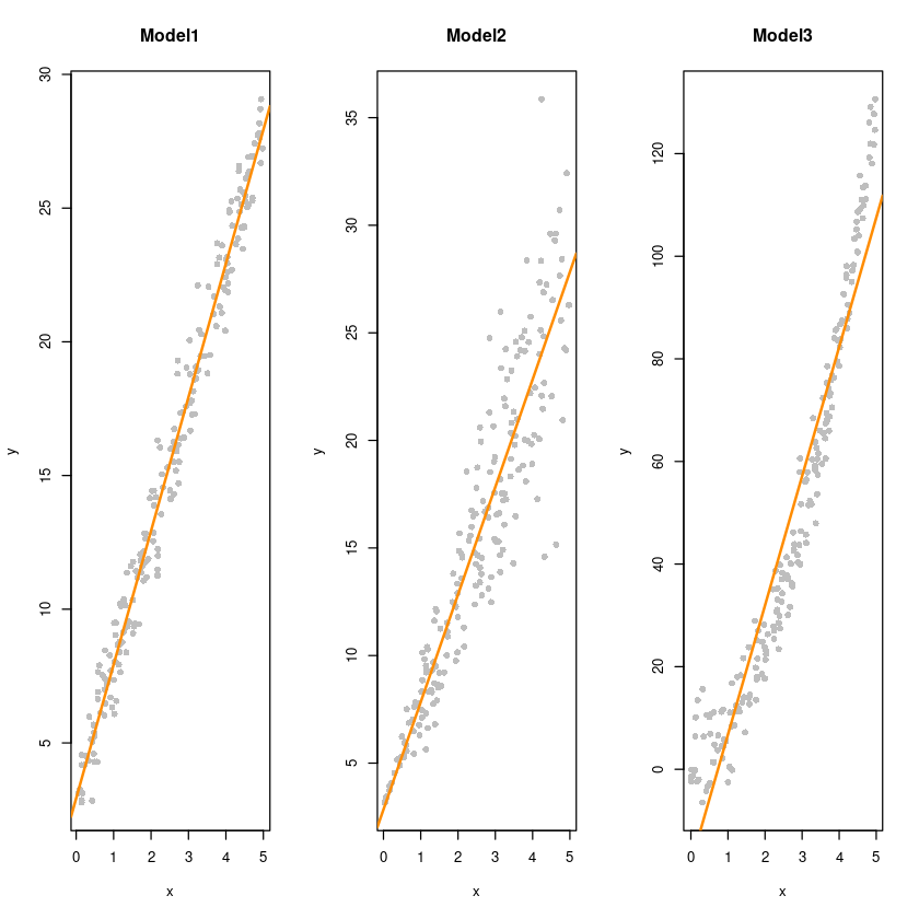
##### residual plot
par(mfrow=c(1,3))
plot(fitted(fit1),resid(fit1), col = 'grey', pch=16,
     xlab = expression(hat(y)),
     ylab = "Residual",
     main = "Residual plot in Model1")
abline(h=0, col='darkorange', lty=2, lwd=2)

# 0에 대해서 대칭인지 확인하자!

plot(fitted(fit2),resid(fit2), col = 'grey', pch=16,
     xlab = expression(hat(y)),
     ylab = "Residual",
     main = "Residual plot in Model2")
abline(h=0, col='darkorange', lty=2, lwd=2)

plot(fitted(fit3),resid(fit3), col = 'grey', pch=16,
     xlab = expression(hat(y)),
     ylab = "Residual",
     main = "Residual plot in Model3")
abline(h=0, col='darkorange', lty=2, lwd=2)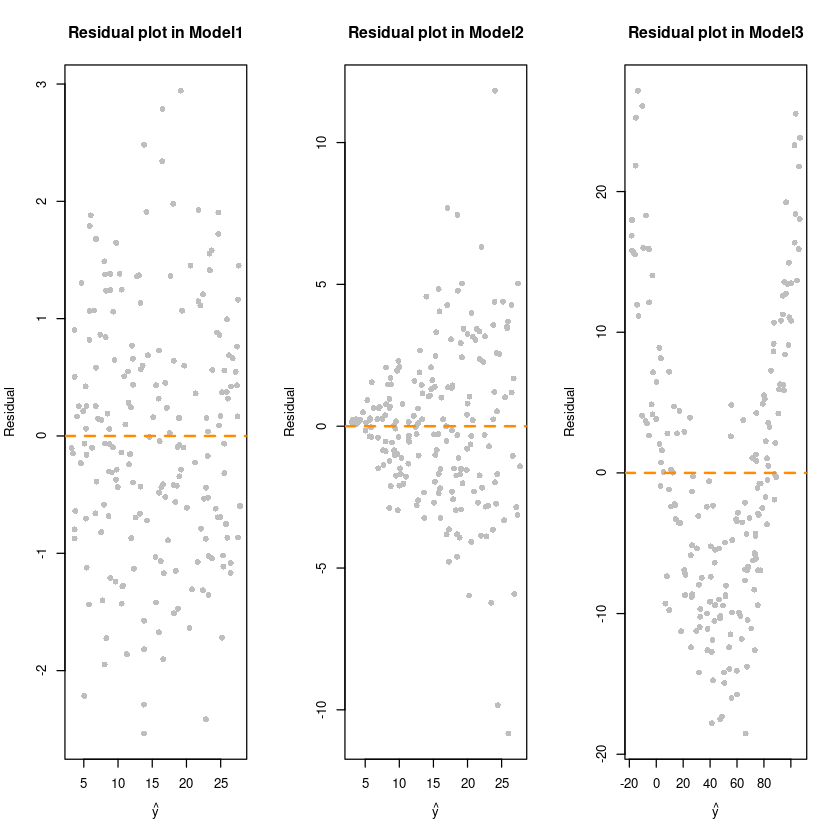
등분산성(homoscedasticity)
#####

### Breusch-Pagan Test
## H0 : 등분산  vs.  H1 : 이분산 (Heteroscedasticity)
library(lmtest)
bptest(fit1) # 0.05보다 큰값이므로 H0를 기각할 수 없다. 등분산
bptest(fit2) # H0기각 이분산이다. (오차에다가 가중치를 사용해서 분산을 안정화시켜줌. x에 비례하도록 가중치를.. 가중최소제곱추정량(WLSE))
bptest(fit3) # H0채택
    studentized Breusch-Pagan test

data:  fit1
BP = 0.11269, df = 1, p-value = 0.7371
    studentized Breusch-Pagan test

data:  fit2
BP = 26.728, df = 1, p-value = 2.342e-07
    studentized Breusch-Pagan test

data:  fit3
BP = 0.19028, df = 1, p-value = 0.6627
정규성 (Normality)
### Histogram of residuals
par(mfrow = c(1, 3))
hist(resid(fit1),
     xlab   = "Residuals",
     main   = "Histogram of Residuals, fit1",
     col    = "darkorange",
     border = "steelblue",
     breaks = 10)
hist(resid(fit2),
     xlab   = "Residuals",
     main   = "Histogram of Residuals, fit2",
     col    = "darkorange",
     border = "steelblue",
     breaks = 10)
hist(resid(fit3),  #오른쪽으로 꼬리가 길다.
     xlab   = "Residuals",
     main   = "Histogram of Residuals, fit3",
     col    = "darkorange",
     border = "steelblue",
     breaks = 10)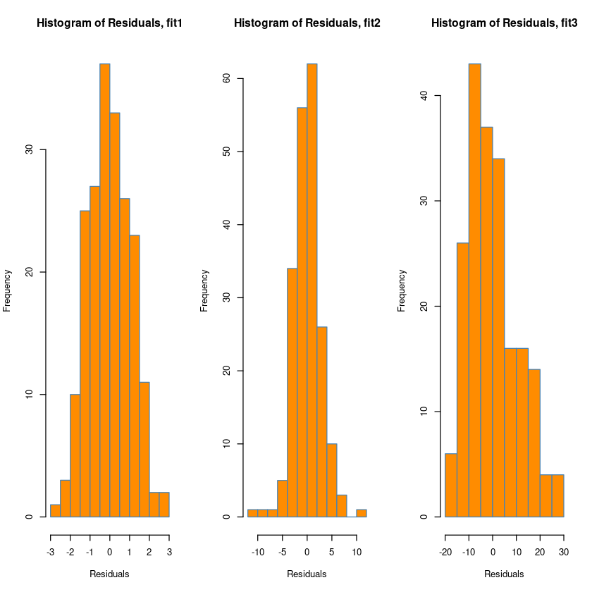
### QQplot
Normal<- rnorm(500)
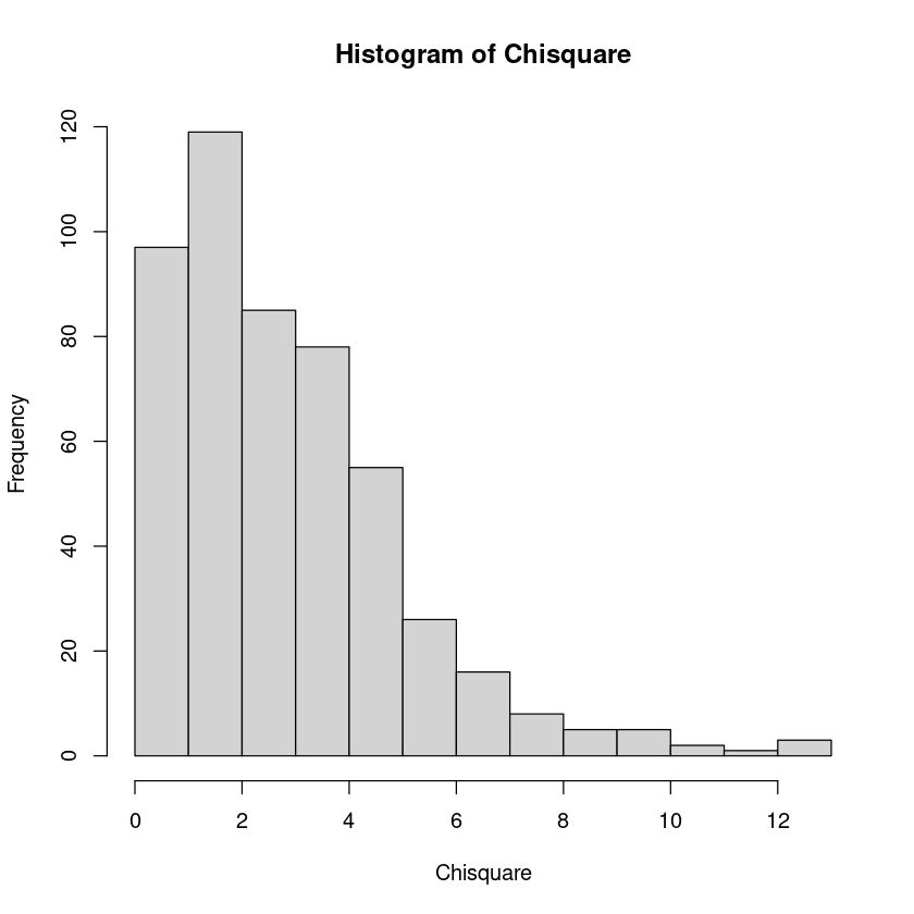
Chisquare <- rchisq(500, 3)
hist(Normal)
hist(Chisquare)
# 빨간색 직선에 붙어있으면 정규분포다.
t2 <- rt(500, 3)par(mfrow=c(1,3))
qqnorm(Normal, pch=16)
qqline(Normal, col = 2, lwd=2)
qqnorm(Chisquare, pch=16)
qqline(Chisquare, col = 2)
qqnorm(t2, pch=16)
qqline(t2, col = 2)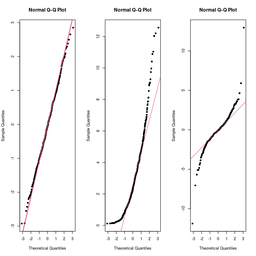
par(mfrow=c(1,3))
hist(Normal, breaks = 10)
hist(Chisquare, breaks = 10)
hist(t2, breaks = 10)
par(mfrow=c(1,1))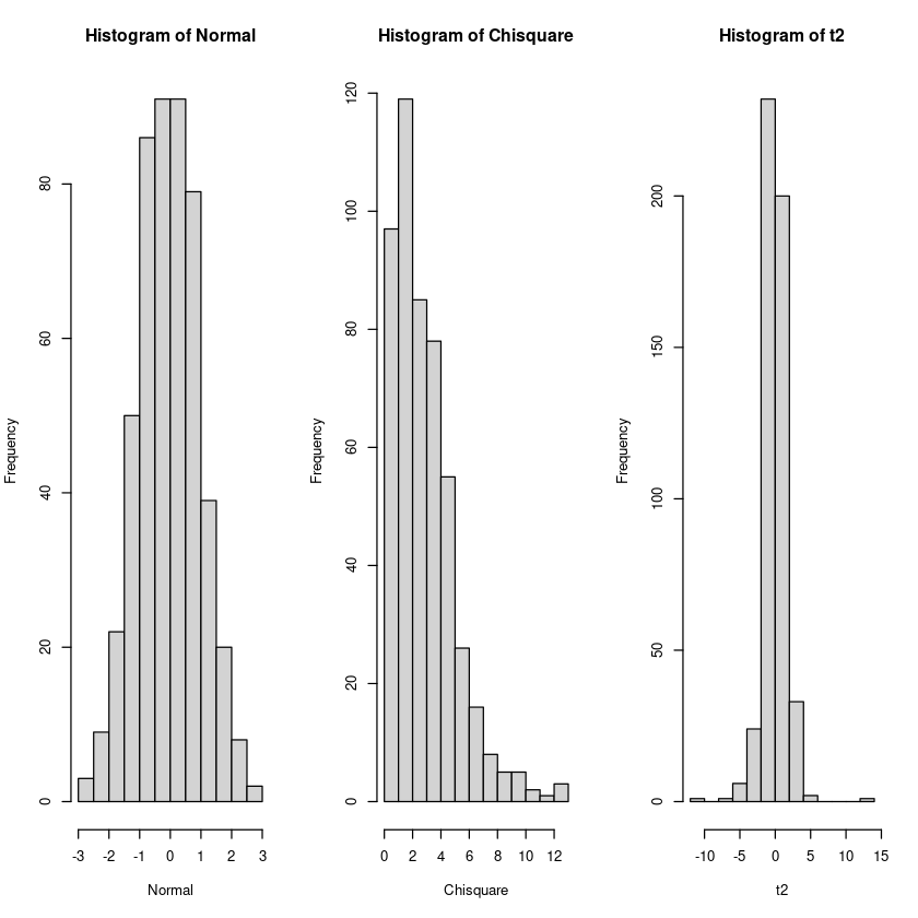
##
par(mfrow=c(1,3))
qqnorm(resid(fit1), main = "Normal Q-Q Plot, fit1", col = "darkgrey")
qqline(resid(fit1), col = "steelblue", lwd = 2)

qqnorm(resid(fit2), main = "Normal Q-Q Plot, fit1", col = "darkgrey")
qqline(resid(fit2), col = "steelblue", lwd = 2)

qqnorm(resid(fit3), main = "Normal Q-Q Plot, fit1", col = "darkgrey")
qqline(resid(fit3), col = "steelblue", lwd = 2)

par(mfrow=c(1,1))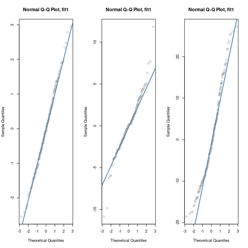
Shapiro-Wilk Test
## H0 : normal distribution  vs. H1 : not H0

shapiro.test(resid(fit1))
shapiro.test(resid(fit2))
shapiro.test(resid(fit3))
    Shapiro-Wilk normality test

data:  resid(fit1)
W = 0.99577, p-value = 0.8555
    Shapiro-Wilk normality test

data:  resid(fit2)
W = 0.96659, p-value = 0.0001095
    Shapiro-Wilk normality test

data:  resid(fit3)
W = 0.96354, p-value = 4.875e-05
독립성 : DW test
library(lmtest)Model4 : y = 3 + 5x + epsilon,
epsilon~N(0, var),correlated
epsilon_i = 0.8 * epsilon_(i-1) + v_i, v_i ~ N(0,1)
sim_4 = function(n) {
  e <- rep(0,n); e[1] <- rnorm(1)

  for(k in 2:n) {
    e[k] <- e[(k-1)]*(0.8) + rnorm(1,0,1)
  } # 오차들이 앞의 오차에 영향을 받고 있어!

  x = runif(n = n) * 5
  y = 3 + 5 * x  + e
  data.frame(x, y)
}
n <- 100
dt4 <- sim_4(n)
fit4 <- lm(y~x, dt4)par(mfrow=c(1,3))
plot(y~x, dt4, col='grey', pch=16, main = "Model4")
abline(fit4, col='darkorange', lwd=2)
plot(fitted(fit4),resid(fit4), col = 'grey', pch=16,
xlab = expression(hat(y)),
ylab = "Residual",
main = "Residual plot in Model4")
abline(h=0, col='darkorange', lty=2, lwd=2)
plot(1:n,resid(fit4), col = 'grey', pch=16, type='l',
xlab = expression(hat(y)),
ylab = "Residual",
main = "Residual plot in Model4")
abline(h=0, col='darkorange', lty=2, lwd=2)
par(mfrow=c(1,1))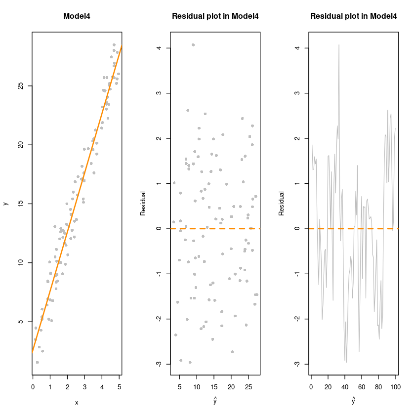
## DWtest
#H0 : 오차들은 독립이다.
dwtest(fit1, alternative = "two.sided")  #H0 : uncorrelated vs H1 : rho != 0
dwtest(fit2, alternative = "two.sided")  #H0 : uncorrelated vs H1 : rho != 0
dwtest(fit3, alternative = "two.sided")  #H0 : uncorrelated vs H1 : rho != 0
dwtest(fit4, alternative = "two.sided")  #H0 : uncorrelated vs H1 : rho != 0
    Durbin-Watson test

data:  fit1
DW = 2.2176, p-value = 0.1241
alternative hypothesis: true autocorrelation is not 0
    Durbin-Watson test

data:  fit2
DW = 2.3155, p-value = 0.02485
alternative hypothesis: true autocorrelation is not 0
    Durbin-Watson test

data:  fit3
DW = 2.1464, p-value = 0.2966
alternative hypothesis: true autocorrelation is not 0
    Durbin-Watson test

data:  fit4
DW = 0.55926, p-value = 3.234e-13
alternative hypothesis: true autocorrelation is not 0
dwtest(fit4, alternative = "two.sided")  #H0 : uncorrelated vs H1 : rho != 0
dwtest(fit4, alternative = "greater")  #H0 : uncorrelated vs H1 : rho > 0 양의상관관계
dwtest(fit4, alternative = "less")     #H0 : uncorrelated vs H1 : rho < 0 음의상관관계


# DW가 4에 가까울수록 음의상관관계가 크고 0에 가까울수록 양의 상관관계가 크다.
    Durbin-Watson test

data:  fit4
DW = 0.55926, p-value = 3.234e-13
alternative hypothesis: true autocorrelation is not 0
    Durbin-Watson test

data:  fit4
DW = 0.55926, p-value = 1.617e-13
alternative hypothesis: true autocorrelation is greater than 0
    Durbin-Watson test

data:  fit4
DW = 0.55926, p-value = 1
alternative hypothesis: true autocorrelation is less than 0